Formation of Cortical Cognitive Map by Self-Organization
저자
: Shun-ichi Amari출처
: Computational Neuroscience , edited by Eric L. Schwartz, The MIT press.1990. pp. 267-277
요약
:뇌의
신경계는 자기조직화에 의해서 외부세계를 뇌 내부에 표현한다고 믿어지고 있다. 즉, 외부세계의 각각의 신호에 반응하는 뉴런의 집단을 형성한다는 것이다. 이러한 뉴런의 집단을 피질인지지도(Cortical cognitive map)라고 부른다. 자기조직화에 의한 정보표현을 연구하는 것은 흥미로운 일이며, 이를 위해 "자기조직신경장"(Self-Organization Neural Field) 모델을 바탕으로 하여 여러 특성을 컴퓨터 시뮬레이션을 이용해서 연구할 수도 있겠지만 본 논문에서는 수학적 분석이 보다 중요함을 강조한다. 수학적 방법에 의하면 case study에 끝나버리는 컴퓨터를 이용한 수치적 방법보다는 "통괄적인 방법" (universal manner)으로 이해할 수 있기 때문이다.
뇌의
자기조직화에 의해 형성된 구조물로 대표적인 것으로 시각계와 체성감각계를 생각할 수 있다. 이들은 정보공간의 모양을 그대로 유지하면서 정보표현을 하고있다. 이런 특성을 topographic organization 이라고 하며, 시각계의 경우 retinotopy, 체성감각계의 경우 somatotopy라고 부른다. 뇌의 시각계는 모양의 정보 요소들인 선분, 방향들을 인지하는 여러 세포군으로 분류되어 있음이 관찰된다. 그러나, 이러한 인지지도는 유정정보 속에 모두 내재되어 있는 것 같지는 않으며, 유전정보에 의해서는 대충의 뉴런간 연결만 형성하며 외부세계의 정보들이 뇌로의 입력과정과 자기조직화에 의해 후천적으로 획득되는 것으로 여겨진다. 또한 시각계의 흥미로운 점 중의 한가지가 3차원 시각정보를 2차원 신경장에 표현할 수 있는 능력인데, 수학적으로는 3차원 공간을 2차원 공간으로 토폴로지를 유지한 채 사상하는 것은 불가능하다. 그러나, 뇌는 이런 문제를 양자화(Quantization)와 미세컬럼구조로 해결하고 있다. 이와 같은 정밀한 구조는 자기조직화와도 관계 있고, 외계 정보구조를 바꾸면 내부구조도 그에 따라 변하는 것으로 알려져 있다.
본
논문에서는 자기조직신경장의 상태(실제로는 전위)를 기술하는 기본방정식을 구성하고, 또한, 헤비안 학습 규칙에 의해 흥분성 결합가중치와 억제성 결합 가중치의 변화를 기술하는 방정식을 구성한다. 이들 두 가지를 기본 방정식으로 하여 다음과 같은 중요한 결론을 제시한다.
1) Amplification Property
"
신호공간에서 신경장에 주어지는 신호의 빈도가 높을수록 신경장에서 형성되는 cognitive -map의 크기가 커진다."2)
Resolution of a Continuous Cognitive Map"신호공간에서 서로 다른 신호를 분류하여 인지 할 수 있는 신경장의 분해능을 제시한다."
3) Law of Constant Activity
"자기조직화는 신경장에 출현하는 신호의 빈도를 동일하게 하려고 한다."
4) Topological Stability of Cognitive Map - Categorization Property
"신경장의 양자화가 나타날 수 있는 조건을 제시하고, 자기조직화에 의해 신경장이 양자화 될 수 있음을 제시한다."
Contents
Introduction
Fundamental Equations of Self-Organizing Neural Fields
Dynamics of Excitation in Neural Fields
Neural Representation of Signals
Self-Organization of Neural Fields
Geometry of Signal Space
Metric Properties of Cognitive Maps
Amplification Property in a Discrete Map
Resolution of a Continuous Cognitive Map
Law of Constant Activity
Amplification Property in Cognitive Map
Conformal Geometry of Cognitive Maps
Topological Stability of Cognitive Map - Categorization Property
Conclusion
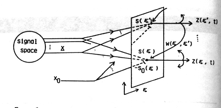
Fundamental Equations of Self-Organizing Neural Fields
Dynamics of Excitation in Neural Fields
수학적
 라고 하자. 그러면 신경장의 어떤 지점 ? , 신간 t에서의 막전위는 다음 식 (1)로써 기술된다.
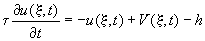
 : The average membrane potential of neurons around position ? at time t.
?
: Time constant.-h : Resting potential.
위치
? 에 있는 뉴런의 평균 출력 펄스의 빈도 는 다음으로 주어진다.

여기서
f는 출력함수라고 불리우며, 시그모이드 함수 또는 간단히 0과 1의 값을 갖는 계단함수 등으로 나타낼 수 있다.한편
, 신경장 내에서 내부결합에 의해 뉴런으로 입력되는 내부 자극은 다음과 같이 주어진다.
한편
외부에서 오는 외부자극은 다음으로 주어진다.


 to the neurons at ? .


.그러면
, 식 (3), (4)를 (1)식에 대입하면 다음이 구해진다.
Neural Representation of Signals
외부에서
입력 가 주어졌을 때 식(5)의 평형상태의 해를
  라고 하면 이는 (5)식에서 시간미분항을 0으로 보내어 다음을 구할 수 있다.

반응영역의
정의 (The response region of signal)

즉
, 신경장에라는 입력이 주어졌을 때 신경장의 위치 ? 에 있는 뉴런의 전위가 양의 값을 갖는 모든 영역을 입력에 의한 신경장의 반응영역이라고 한다.
신호수용역의
정의 (Receptive field of the neurons at ? ,)
즉
, 신경장의 위치 ? 에 있는 뉴런의 전위가 양의 값을 갖게하는 신호공간의 모든 입력를 ? 의 신호수용영역이라고 한다.
Self-Organization of Neural Fields
Hebbian rule:



식
(7)은 흥분성 입력신호에 곱해지는 결합효율(가중치)이고 식(8)은 억제성 신호 에 곱해지는 결합효율(가중치)이다.
식
(4)를 미분하고 (7)과 (8)을 대입하면 다음을 얻는다.

여기서
수학적 취급의 간편함을 위해서 x0 를 상수로 둔다.이제
신호공간에서 확률 p(x)를 지닌 신호들이 무작위로 신경장 F 에 주어지는 경우를 생각한다.그러면
x에 대한 평균 방정식은 다음으로 주어진다.

그리고
, 평형 방정식은 다음으로 주어진다.

식
(9)를 평균취하면,
여기서
 (14)
(14)
최종적인
평균화 평형 방정식은 다음으로 주어진다.
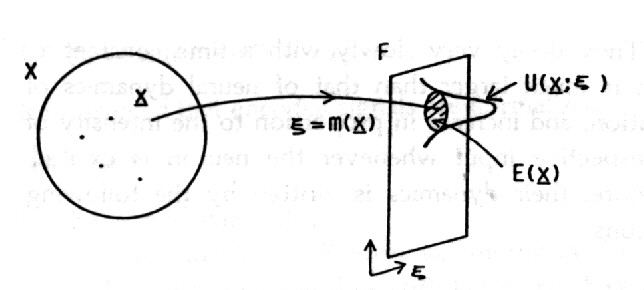
Geometry of Signal Space
Signal space is an n-dimensional vector space. In some case, not all of the in signal space are applied to F but only a small part is used as environmental signals.
We call  a signal set and then they are represented by neural excitations at positions
  . Let pi (i=1,…,m) be the probability of occurrence of signal
  .Then,
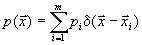
The geometrical relations between two signals are given by

Although we do not know the position ? I of the cognitive map, we can show some properties of neural representation, e.g., the amplification property that a large region is assigned to a signal appearing frequency.
Let us introduce an m-dimensional coordinate system  in S to specify a signal. That is, a signal specified by ? is denoted by
  . The simplest example is the case where positional information ? denotes positions of some space. It is mathematically tractable to study in F when ? is continuous.

it is assumed that encoded signals are normalized,

Now we introduce a Riemannian metric in S that is induced by the encoding  . Let ds be the length between two adjacent signal ? and ? +d? . We define ds by the Euclidean length in X,
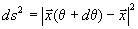
By using the normalization condition (17), we have


Let
 (20)
(20)
Then the volume of a small region is measured by  (21)
(21)
Let p(? ) be the probability density of signal  ,
, (22)(invariant under any coordinate - transformation)
The probability of a signal appearing in a region d? is given by  . It should be remarked that p(? ) and
  play a similar role in the formation of a cognitive map.A homogeneous field F is considered to be a Euclidean space. It is interesting to know how a Riemannian manifold S is mapped in a Euclidean field F by self-organization.
Metric Properties of Cognitive Maps
Amplification Property
신호공간
S 가 m 개의 신호 으로 구성되어 있다고 하자. 그러면, 식 (15)는 다음으로 변형된다.

여기서
,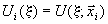 이며, x 에 의한 발화패턴이다. m개의 신호가 뜨문뜨문 배치되어 있고, 신호반응영역이 서로 중첩되지 않는 경우에는 위의 식은 다음으로 간단히 나타난다.

이제
여기서 보이고자 하는 것은 자주 보여주는 신호에 의한 신호반응영역의 크기가 증대되는 현상이다. 이를 amplification property라고 한다. 이를 보이기 위해 먼저 신경장 F가 1차원인 경우를 고려한다. 그리고 를 ? = 0 주변의 폭 a를 갖는 경우를 생각한다. 그러면 식 (23)은 다음과 같이 나타낼수 있다.

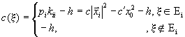
여기서
,
또한
, .
.
신경장의
반응영역 폭 a 는 의 조건에서 구해지며, 다음과 같다.
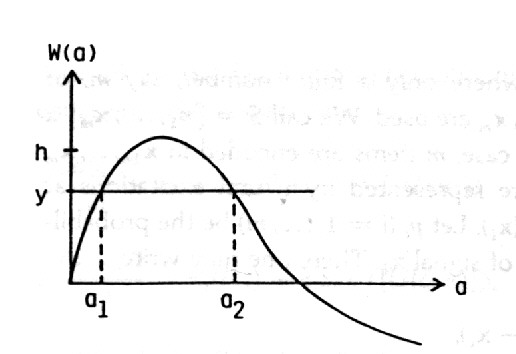

where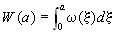 (25)
(25)
식
(24)의 우변이 0이 되는 조건에서 a 값은 다음그림과 같이 ,
,  의 교점의 x좌표값을 구하면 된다. 두개의 해가 존재하지만, 큰 값이 안정해 임이 보여졌다 [Amari 1977]. 주어지는 신호의 확률이 큰 값인 경우에는 직선 는 아래로 내려오고 교점의 값은 더욱 큰 값을 갖게 된다. 즉, 자주 보여지는 신호가 뇌 내에서 많은 영역을 차지하게 됨을 보여준다.
(다음 문장에서는 영문으로 작성되어 있습니다. 한글로 바꿀 계획입니다.)
Resolution of a Continuous Cognitive Map
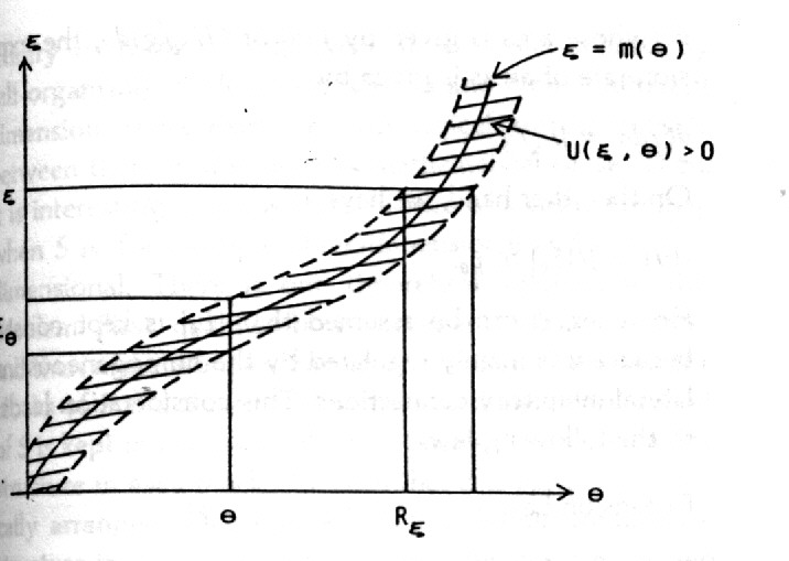
We study the case where S is a two-dimensional continuous set for the purpose of understanding how signal mutually interact to form a cognitive map. Let us assume that a topological map  is formed between two 2-dimensional field S and F. This means that the final equilibrium solution
  takes its maximum, for each fixed ? , at .
The response region

Receptive field


Where and  .
.
The efficacy of x0 at the equilibrium is given by

When f is unit step function, it is proportional to the average firing frequency  of neurons at ? . Since it is given by the probability
  that a signal x is included in the receptive field
  , where
  , we have

On the other hand,

where the average is taken over  . Hence, the term
  attains its maximum at , when ? is fixed. Since
  itself attains its maximum at , this implies that should be a constant function in the equilibrium.
Law of constant activity
"Self-organization has a tendency of letting all the neurons be excited equally frequently."
Now we consider resolution of a cognitive map. Let us consider a small region d? in S, and let  be the maximum number of signals in d? whose response regions do not overlap in F. Obviously
 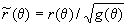 is an invariant,
  giving the number of distinguishable signal. Since region d? is mapped to
  , and an excitation pattern occupies an area
  , this number is given by
  . Because of (29) and =const., we have
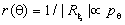
In terms of invariant resolution
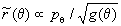
Thus we have resolution law.
Resolution Law
"The resolution of signals at ? is proportional to the relative frequency of signals around ? , and is in inverse proportion to the volume density  ."
."
Conformal Geometry of Cognitive Maps
Let us pick up a number of signals in S randomly in proportion to the probability density  and apply only these selected signals, in order to see the positions where these signals represented in F. We have
  signals in a small region
  .
.
The expansion rate of areas is given by

Expansion Law.
"The rate of local expansion of S in the cognitive map is proportional to the invariant frequency."
Topological Stability of Cognitive Map - Categorization Property
When S and F have different dimension, there exists no topological correspondence between them in the rigorous mathematical sense. Then, it is interesting to know the structure of a cognitive map when S is, for example, 3-dimensional and F is 2-dimensional.
In order to study the stability of the continuous equilibrium solution  of the field equations (15), we need to write down the variational equation,
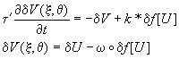
around the equilibrium  .
.
The solution is stable when the operator  has no eigenvalues whose real part is great than 1. However, it is difficult to check it. When S and F are one dimensional and homogeneous, the equilibrium solution has the following form

with the linear cognitive map  . When f is approximated by the step function, we denote the equilibrium excited region by the interval

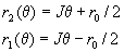
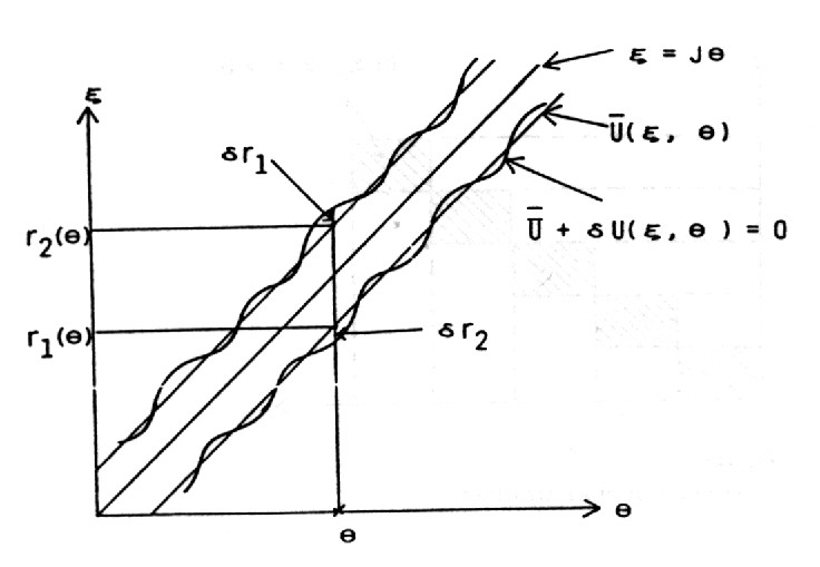
A small variation causes a change in the boundaries to yield new boundries

We rewrite the variational equation (36) in terms of the variations  to yield a set of differential difference equations. We do not discuss the technical details, but we can prove the following theorem.
Theorem
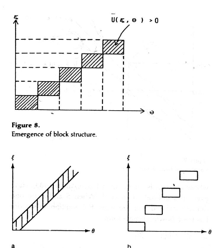
"The continuous map is stable when  , and is unstable when
  , where r0 is the length of the receptive field determined from

When the continuous map is stable, the representation changes continuously in ? . However, when it is unstable, the mathematical analyses of the variational equations do not tell us the possible cognitive map. A computer simulated experiment shows that a block structure emerges in this case, as shown in fig .8.
References
Amari,S. (1972) Learning patterns and pattern sequences by self organizing nets of threshold elements. IEEE Trans. c-21: 1197-1206.
Amari,S. (1977) Dynamics of pattern formation in lateral-inhibition type neural fields. Biol. Cybern. 27: 77-87.
Amari,S. (1980) Topographic organization of nerve fields. BulL. Math.BioL 42: 339-364.
Amari,S. (1983) Field theory of self organizing neural nets. IEEE Tnas. SMC-13: 741-748.
Amari,S. and Takeuchi. A. (1978) Mathematical theory on fonTLation olcategory detecting nerve cells. Biol. Cybern. 29: 127-136.
Anderson, J. A. (1972) Simple neural network generating interactive memory. Math. Biosci. 14:194-220.
Birnenstock E. L. Cooper. L N. and Munro. P. W. (1982) Theory for the development of neuron selectivity: Orientation specificity and binocular interaction in visual cortex. J. Neurosci. 2: 32-48.
Cohen , L.N. and Grossberg, S. (1983) Absolute stability of global pattern formation and parallel memory storage by competitive neural network. IEEE Trans. SMC-13: 815-626.
Cooper. L N.. Lieberman. F. and Oja, E. (1979) A theory for the acquisition and loss of neuron specificity in visual c3rtex. Biol. Cybern.
33: 9-28.
Hopfield,J.J. (1982) Neural networks and physical Systems with emergent Collective computational abilities. Proc. Natl. Acad. Sci. USA 79: 2445-2558.
Kohoren T. (1977) Associative Memory, Springer, New York.
Kohonen. T. (1984) Self- Organization and Associative Memory. Springer. New York
Nakano. K. (1972) Associatron - a model of associative memory. IEEE Trans. SMC-2: 351-388.
Rumelhart. D.E., McClelland, J. L. et al. (1986) Parallel Distributed Processing. vols 1.2 MIT Press. Cambridge.
Takeuchi, A.. and Arnari. S. (1979) Formation of topographic maps and columnar microstructures. Biol. Cybern. 35: 63-72.
von der Malsburg. C. (1973) Self-organization of orientation sensitive cells in the striate cortex. Kybernetik 14: 85-100.
Willshaw, D. J. and von der Malsburg C. (1976) How patterned neural connections can be set up by self-organization. Proc. Roy. Soc. London
194: 431-445.